Typically you have many tables of data, and you must combine them to answer the questions that you’re interested in.
Collectively, multiple tables of data are called relational data because it is the relations, not just the individual datasets, that are important.
Relations are always defined between a pair of tables.
Verbs that work with pairs of tables
There are three families of verbs designed to work with relational data:
Mutating joins, which add new variables to one data frame from matching observations in another.
Filtering joins, which filter observations from one data frame based on whether or not they match an observation in the other table.
Set operations, which treat observations as if they were set elements.
Prerequisites
The most common place to find relational data is in a relational database management system.
If you’ve used a database before, you’ve almost certainly used SQL.
We will explore relational data from nycflights13 using the two-table verbs from dplyr.
library(tidyverse)library(nycflights13)
Workshop Part 1: INTRODUCTION TO RELATIONAL DATA
?nycflights13
nycflights13 contains four tibbles
airlines lets you look up the full carrier name from its abbreviated carrier code
airports gives information about each airport, identified by the faa airport code
planes gives information about each plane, identified by its tailnum
weather gives the weather at each NYC airport for each hour
EXERCISE
Examine the variables that exist across the 4 tibbles in nycflights13 and draw a diagram depicting the relationships that exists between flights and the other tables.
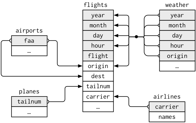
Relationships with flights
flights connects to planes via a single variable, tailnum
flights connects to airlines through the carrier variable
flights connects to airports in two ways: via the origin and dest variables
flights connects to weather via origin, and year, month, day and hour variables
Relationships in nycflights13
Questions
What is the relationship between weather and airports and how should it appear in the diagram?
Weather only contains information for the origin (NYC) airports. If it contained weather records for all airports in the USA, what additional relation would it define with flights?
We know that some days of the year are “special”, and fewer people than usual fly on them. How might you represent that data as a data frame? How would it connect to the existing tables?
What is a key?
A key is a variable (or set of variables) that uniquely identifies an observation.
A primary key uniquely identifies an observation in its own table. For example, planes$tailnum is a primary key because it uniquely identifies each plane in the planes table.
A foreign key uniquely identifies an observation in another table. For example, flights$tailnum is a foreign key because it appears in the flights table where it matches each flight to a unique plane.
EXERCISE
Identify the primary keys across the tables.
How can we check this?
dataset |>count(var) |>filter(n >1)
Surrogate key
It is clear that flights does not have an explicit primary key.
If a table lacks a primary key, it’s sometimes useful to add one with mutate() and row_number().
This is called a surrogate key and makes it easier to check back with the original data following manipulation.
Identifying keys
A primary key and the corresponding foreign key in another table form a relation.
In simple cases, a single variable is sufficient to identify an observation (plane: tailnum).
In other cases, multiple variables may be needed (weather: year, month, day, hour, origin).
Relations are typically one-to-many. For example, each flight has one plane, but each plane has many flights.
Workshop Part 2: Mutating Joins
A mutating join allows you to combine variables from two tables. It first matches observations by their keys, then copies across variables from one table to the other.
Understanding joins
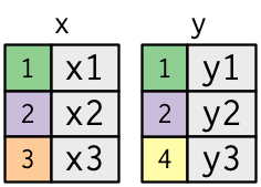
To help us understand joins, let’s create the following two tables.
The coloured column represents the “key” variable: these are used to match the rows between the tables.
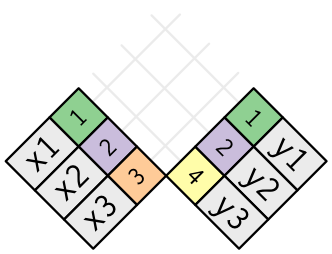
Understanding joins
In an actual join, matches will be indicated with dots. The number of dots = the number of matches = the number of rows in the output.
Understanding joins
In an actual join, matches will be indicated with dots. The number of dots = the number of matches = the number of rows in the output.
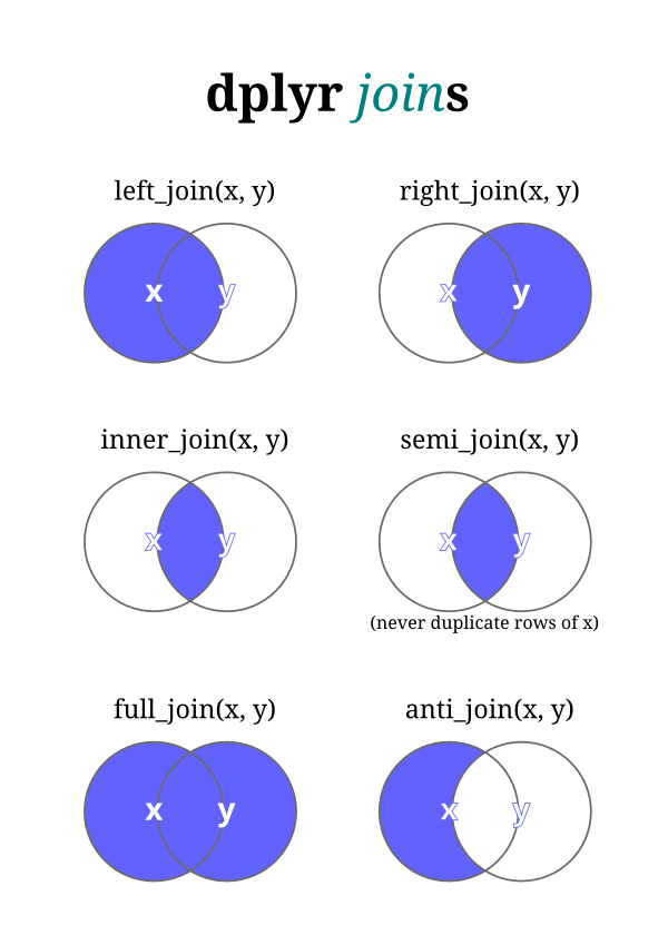
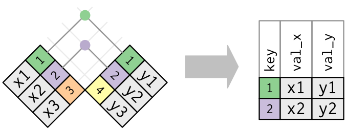
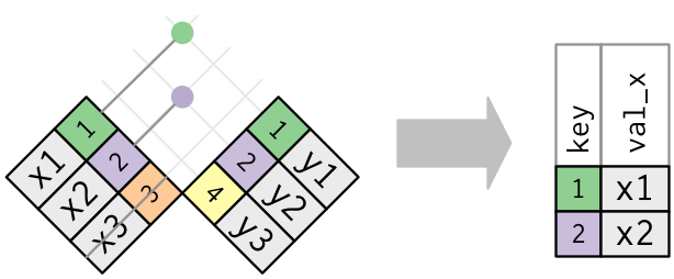
inner_join
The simplest type of join is the inner join. An inner join matches pairs of observations whenever their keys are equal. We use by to tell dplyr which variable is the key.
x |>inner_join(y, by ="key")
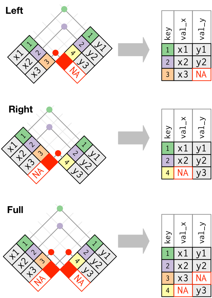
outer_join
An outer join keeps observations that appear in at least one of the tables. There are three types of outer joins:
A left join keeps all observations in x.
A right join keeps all observations in y.
A full join keeps all observations in x and y.
outer_join
left_join()
Imagine you want to add the full airline name to the flights data. You can combine the airlines and flights data frames with left_join().
flights |>select(-origin, -dest) |>left_join(airlines, by ="carrier")
EXERCISE
Explore the different outer join options across the tables.
Duplicate keys
So far all the diagrams have assumed that the keys are unique. There are two possibilities when keys are not unique.
One table has duplicate keys
Both tables have duplicate keys
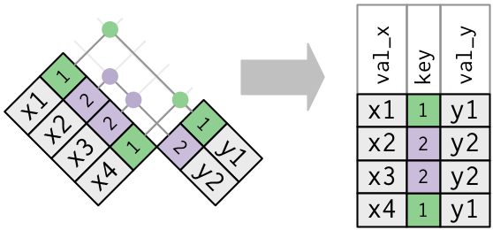
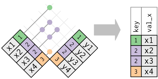
One table - Duplicate keys
This is useful when you want to add in additional information as there is typically a one-to-many relationship.
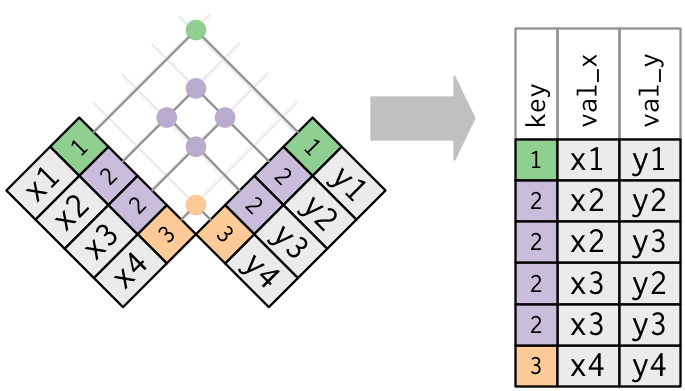
Both tables - Duplicate keys
When you join duplicated keys, you get all possible combinations.
Natural joins
You can use other values for by to connect the tables in other ways:
The default, by = NULL, uses all variables that appear in both tables, the so called natural join.
A character vector, by = "x". This is like a natural join, but uses only some of the common variables.
A named character vector: by = c("a" = "b"). This will match variable a in table x to variable b in table y. The variables from x will be used in the output.
Workshop Part 3: Filtering Joins
Filtering joins match observations in the same way as mutating joins, but affect the observations, not the variables. There are two types:
semi_join(x, y) keeps all observations in x that have a match in y.
anti_join(x, y) drops all observations in x that have a match in y.
Filtering joins
Semi-joins are useful for matching filtered summary tables back to the original rows. For example, imagine you’ve found the top ten most popular destinations.
Now you want to find each flight that went to one of those destinations. You could construct a filter yourself.
flights |>filter(dest %in% top_dest$dest)
Semi-joins
Instead you can use a semi-join, which connects the two tables like a mutating join, but instead of adding new columns, only keeps the rows in x that have a match in y.
flights |>semi_join(top_dest)
Semi-joins
Graphically, a semi-join looks like this:
Semi-joins
Only the existence of a match is important; it doesn’t matter which observation is matched. This means that filtering joins never duplicate rows like mutating joins do.
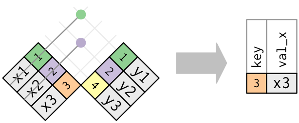
Anti-joins
The inverse of a semi-join is an anti-join. An anti-join keeps the rows that don’t have a match.
Anti-joins
Anti-joins are useful for diagnosing join mismatches. For example, when connecting flights and planes, you might be interested to know that there are many flights that don’t have a match in planes.
flights |>anti_join(planes, by ="tailnum") |>count(tailnum, sort =TRUE)
Set Operations
The final type of two-table verb are the set operations. All these operations work with a complete row, comparing the values of every variable. These expect the x and y inputs to have the same variables:
intersect(x, y): return only observations in both x and y.
union(x, y): return unique observations in x and y.
setdiff(x, y): return observations in x, but not in y.